
RLiG learns the structure of a Bayesian network with reinforcement learning. An agent edits a graph one edge at a time, and its reward mixes the usual BIC score with a second score for how well the learned network generates data. That second score is expensive, so the agent only pays for it at chosen steps. I wrote this up as the High Distinction task for SIT320 Advanced Algorithms at Deakin in T2 2026. This post is that paper, shortened, with the marking parts taken out.
The unit's task sheet set the RLiG problem: the hybrid reward, the tiles and the baselines. My part was the implementation, the difference-form reward, the β calibration, the agents and the experiments.
The headline is a negative result, and I think it is the most useful part. The expensive half of the reward, which is the part I could not find in the literature, mostly did not help. What did well was the linear agent with the generative half switched off.
The problem
A Bayesian network is a directed acyclic graph (a DAG) over some variables, plus a probability table for each variable given its parents. Learning the structure means finding the graph from data. The normal way is a greedy search over DAGs: add, delete or reverse whichever edge improves a score like BIC the most, and stop when nothing improves it. Nothing but the score guides it.
RLiG changes two things. It turns the search into a sequential decision problem, so an edit can be worth making even when it lowers the score right now. And it adds a second term that asks how good the network is at the job it often gets built for, which is generating realistic data.
The decision process
Given N rows of discrete data over d variables:
- State. The current DAG as a boolean adjacency matrix, the position inside the tile (t mod L), and a few summary numbers: BIC per row, edge count, progress through the episode, in-degree, a stall counter, the last measured generative score and how much of the generative budget is spent.
- Actions. (op, i, j) with op one of add, delete or reverse, so 3d2 in the raw encoding. An action is legal only if the graph stays acyclic and no node gets more than k parents.
- Episodes end after T edits, or after 15 steps with no BIC improvement.
Write BICN for BIC divided by the number of rows, and Gen(G) for the generation score, which sits between 0 and 1. The hybrid score is:
At an ordinary step the reward is just the change in α · BICN. At a generative step it also adds β times the change in Gen since the last generative step, because Gen was never measured on the graph in between.
Why the reward is a difference
With no discounting (γ = 1) a difference reward telescopes. Add up every step and the BIC part collapses to the change from the first graph to the last. So maximising the return is close to maximising the hybrid score of the final graph. That is the whole reason to use RL here. An edit that lowers the score is allowed, it just has to be paid back before the episode ends, and a greedy hill climber cannot do that at all. A test in the notebook checks this identity to six decimal places.
It is not quite the clean H(GT) − H(G0), for two reasons. Gen is never measured on the starting graph, so the first measured graph becomes the baseline. And with tiles, the generative part only telescopes between generative steps.
Tiles, and what they save
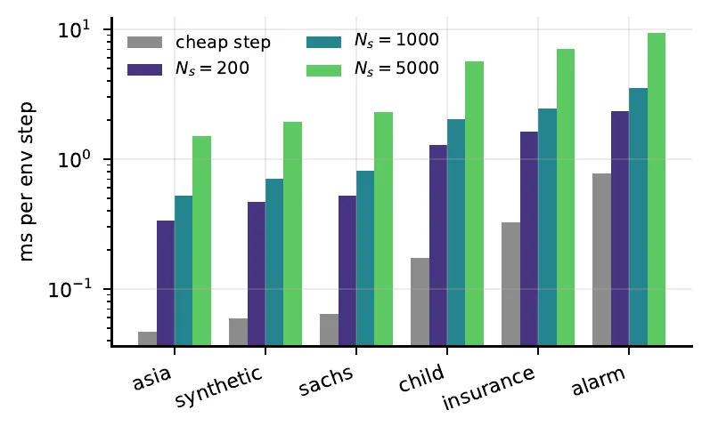
Step t is generative when t mod L is in a set Ig. With L = 5, Ig = {0} and T = 40, an episode schedules eight simulate-and-compare calls instead of forty. A cheap step is a cached BIC change for each legal action, while a generative step also has to fit the probability tables, simulate Ns rows and compare them with real data. I timed both.
view data
| category | Cheap step | Generative step |
|---|---|---|
| synthetic | 0.06 ms | 0.71 ms |
| asia | 0.05 ms | 0.52 ms |
| sachs | 0.08 ms | 0.81 ms |
| child | 0.16 ms | 2.02 ms |
| insurance | 0.29 ms | 2.44 ms |
| alarm | 0.77 ms | 3.51 ms |
| Network | d | Cheap step (ms) | Generative step (ms) | Ratio |
|---|---|---|---|---|
| synthetic | 10 | 0.06 | 0.71 | 12.0× |
| asia | 8 | 0.05 | 0.52 | 10.5× |
| sachs | 11 | 0.08 | 0.81 | 10.5× |
| child | 20 | 0.16 | 2.02 | 12.9× |
| insurance | 27 | 0.29 | 2.44 | 8.3× |
| alarm | 37 | 0.77 | 3.51 | 4.5× |
Those timings use Ns = 1000. The main runs simulate 5000 rows, where the ratio reaches 36× on Child. That ratio shrinks on the widest network because a cheap step has to score every legal edit, and ALARM has a lot of them. Tiling therefore pays best on smaller networks and big simulations.
The two halves of the score
BIC splits into one term per variable and its parents. That split is the only reason any of this runs fast, because an edit touches one family (two for a reversal) and every family score is cached:
Gen(G) fits every probability table on the training rows with a Dirichlet prior of 1, simulates Ns rows, and compares the one-way and two-way marginals against a held-out reference split using Jensen-Shannon divergence in bits (Lin, 1991). Its value is 1 minus the average divergence. JS in bits is bounded by 1, so Gen stays between 0 and 1 whatever the number of variables. I hold the reference split out on purpose. Scoring a simulation against the rows its own tables were fitted to would reward a graph for copying noise.
Calibrating β
The two halves turned out to be about two orders of magnitude apart, which I did not expect. On ASIA at 500 rows, going from the empty graph to hill climbing's graph moves BICN by about 0.65 and Gen by about 0.0062. At α = β = 1 the generative term would do nothing, and a sweep over β would look like it measured something when it did not. For each dataset I set:
Every run quotes β as a multiple ρ of that. ρ = 1 is balanced by construction, and I fixed it before looking at any result. The ρ = 0 rows were added after the sweep, once ρ = 0 kept doing better. β* comes out at about 104 on ASIA and about 1837 on ALARM, which is why a raw β cannot carry across networks but ρ can.
Three agents
- Tabular Q-learning (Watkins and Dayan, 1992), keyed on the graph bytes and the tile position. Exact, and only feasible while the table stays small.
- Linear Q over fifteen hand-built features. Anything that is the same for every action in a state cannot change which action wins, so state variables only appear multiplied by something that varies, like the BIC change of that action.
- A DQN (Mnih et al., 2015) with learned embeddings for i, j and the operator, so one network covers any edit at any graph width. Illegal actions are masked before the argmax and before the bootstrap max (Huang and Ontañón, 2022), so it never has to learn acyclicity.
The BIC change is an input feature for both learned agents on purpose. RLiG only has to learn when following the score is the wrong move. I expected uniform exploration to waste steps, since a sparse ALARM graph offers roughly thirteen hundred legal edits, so RLiG explores with a Boltzmann draw over the BIC change. In the small two-seed ablation, uniform was actually ahead on ASIA and Child, so that choice is untested.
One episode, as pseudocode:
G <- init()                          # empty, random, or a hill-climb warm start
for t = 0 .. T-1:
    A <- feasible_edits(G)           # cycle and in-degree masks off one closure
    D <- bic_deltas(G, A)            # cached local scores, two for a reversal
    a <- policy(s_t, A, D)           # argmax on Q, Boltzmann on D when exploring
    G' <- apply(a, G)
    if (t mod L) in I_g:             # or the meta-head says spend, and budget remains
        r <- alpha*dBIC_N + beta*(Gen(G')-g_last)  # N_s rows from G', compare
        remember (H(G'), G')         # only measured graphs can be the answer
    else:
        r <- alpha * (BIC_N(G') - BIC_N(G))
    update(s_t, a, r, s_{t+1});  G <- G'
return the graph with the best measured H
The last line matters more than it looks. Only graphs seen at a generative step can be returned, so with L = 5 the answer comes from one in five of the graphs visited.
Setup
Five discrete benchmark networks from the bnlearn Bayesian Network Repository (Scutari), plus one synthetic network with a known true graph. None of it is real-world data. Each network gets one sampled dataset: 500 rows to fit the tables and the BIC, 2000 as the reference for Gen, and 5000 held out for the final metrics only. 500 training rows is deliberate. With 5000 rows BIC is close to consistent on these networks and a second objective has little left to add.
| Network | Variables | Arcs | Max parents | β* |
|---|---|---|---|---|
| synthetic | 10 | 12 | 3 | 166 |
| asia (Lauritzen and Spiegelhalter, 1988) | 8 | 8 | 2 | 104 |
| sachs (Sachs et al., 2005) | 11 | 17 | 3 | 145 |
| child | 20 | 25 | 2 | 523 |
| insurance (Binder et al., 1997) | 27 | 52 | 3 | 1016 |
| alarm (Beinlich et al., 1989) | 37 | 46 | 4 | 1837 |
The in-degree cap is k = 3. ALARM has a node with four parents, so its true graph is out of reach for every capped method, and a non-zero error is forced there.
I wrote all four baselines myself, because the searchers are the thing being compared: hill climbing on BIC, the same with a tabu list, GES following Chickering (2002) with Meek's orientation rules (Meek, 1995), and PC with a G² test (Spirtes et al., 2000). My GES has two stated deviations from Chickering. It only enumerates subsets up to size three, and its delete step respects the in-degree cap. My notebook has 55 tests that run in 2.4 seconds. They include checking the action masks against applying every edit for real, and checking the equivalence-class code against every DAG on three, four and five nodes, which is 29281 graphs at five.
Structure is scored as structural Hamming distance (SHD) on the equivalence class, the way Tsamardinos et al. (2006) define it. A reversed edge that the data cannot tell apart costs nothing. Lower is better. Each learned agent runs ten seeds. One dataset is drawn per network and every method sees the same draw, so a seed changes the agent and not the data.
Results
SHD on the equivalence class, mean ± one standard deviation over ten seeds where it varies. ρ = 1 is the hybrid reward. ρ = 0 switches the generative half off.
| Network | Hill climb | GES | PC | Linear, ρ=0 | Linear, ρ=1 | DQN, ρ=0 |
|---|---|---|---|---|---|---|
| synthetic | 5.0 | 4.0 | 11.0 | 1.0 | 2.7 ± 2.3 | 1.0 |
| asia | 4.0 | 5.0 | 8.0 | 1.0 | 3.4 ± 2.2 | 1.0 |
| sachs | 5.0 | 13.0 | 7.0 | 13.0 | 7.2 ± 2.6 | 13.0 |
| child | 18.0 | 13.0 | 21.0 | 13.0 | 12.4 ± 1.6 | 20.3 ± 3.7 |
| insurance | 40.0 | 36.0 | 46.0 | 35.2 ± 1.0 | 37.7 ± 4.5 | 51.2 ± 3.6 |
| alarm | 41.0 | 31.0 | 34.0 | 36.4 ± 2.7 | 41.5 ± 3.8 | 47.8 ± 2.6 |
With the generative half off, the linear agent is the best structure learner in the table on three of six networks, sharing first place with the DQN on two of them. On the synthetic network and ASIA it hits SHD 1.0 on every seed, where hill climbing and GES are four or five off. Its ASIA graph even has a better BIC than the true graph, −1107 against −1110. Insurance goes its way too, 35.2 against 36.0 for GES, but that gap is smaller than its own seed spread.
It does not come first on the other three: it loses ALARM and Sachs and ties Child. On ALARM, GES is clearly ahead at 31.0, and that is the one clean win for equivalence-class search here. Child ends in a tie: the agent lands in GES's equivalence class on every seed, same BIC and same SHD of 13.0. Child is also the one place the hybrid at ρ = 1 beats every other method, 12.4 against 13.0, but that is inside its spread and beats 13 on only four seeds of ten, so I would not lean on it.
On Sachs, hill climbing gets SHD 5.0 at a BIC of −4066. GES and the ρ = 0 agent both find the better BIC of −4062 and both land on 13.0. Two unrelated searches reaching a better score and the same worse graph points at the score itself at this sample size, though it does not prove they returned the same graph. Here the ρ = 1 runs do better, 7.2 ± 2.6 for the linear agent and 8.4 ± 3.2 for the DQN, against 13.0 on every seed at ρ = 0. That gap is larger than the seed spread, so it is the one clear structural gain from the generative half, and it cuts against my headline. My ρ sweep did not cover Sachs, so I cannot say much more.
The DQN is the weakest agent, and it loses on the wide networks. At ρ = 0 it matches the linear agent on the three smallest, then falls to 51.2 on Insurance and 47.8 on ALARM. ALARM gives it about 13000 gradient steps for about 15000 parameters, and its bootstrap target only looks at a shortlist of 24 actions out of about 1300. Both are fixable with compute. The linear agent's fifteen features may also be a strong built-in bias that happens to land close to right, and I cannot tell how much of the gap that explains.
Learning curves
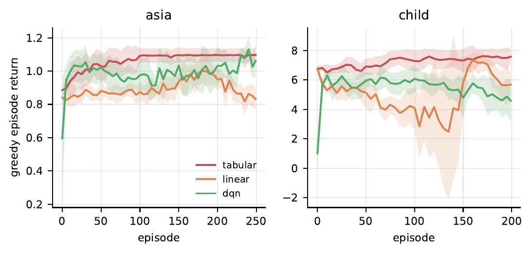
By episode 100 the tabular curve on ASIA has climbed to about 1.10, and after that it barely moves. Tabular finishes highest on both, but its table grows fast: about 490 distinct states on ASIA against about 4800 on Child, so it will not scale far past that.
Does the generative half help?
I swept ρ from 0 to 4 on three networks with two agents, ten seeds each, to find out.
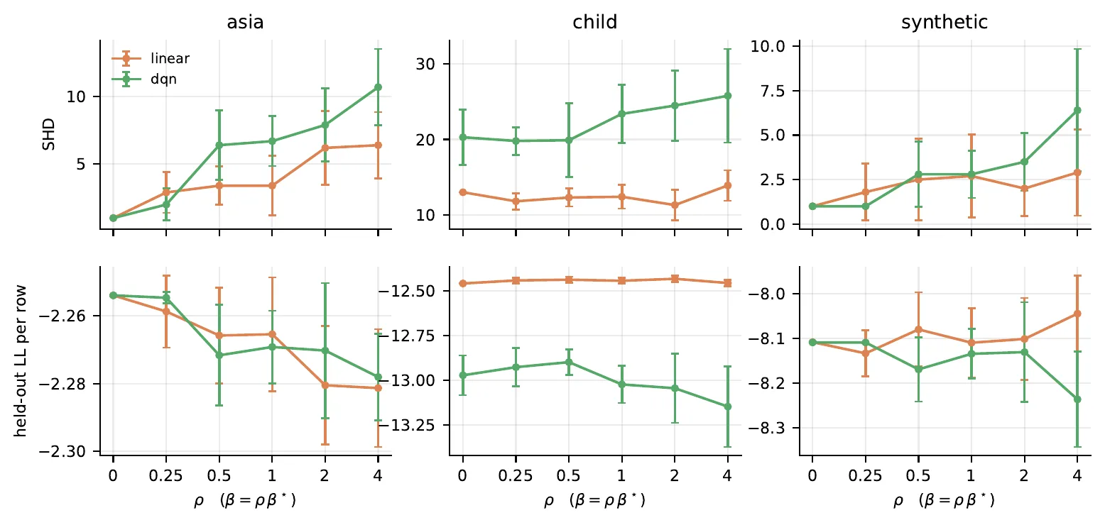
Mostly it does not. Four of the six curves have their best SHD at ρ = 0. Both exceptions are Child: the linear agent is flat and noisy across the whole range, 11.3 to 13.9, and the DQN's best point sits inside its own ρ = 0 spread. Two-way JS is the thing the generative half is meant to improve. Five of six curves do best above zero, but no gap clears the seed spread.
I expected a trade-off, with better generation bought with worse structure. One seed at a smaller budget seemed to show it. Ten seeds did not.
Why the marginal score is too flat
Gen averages divergences over one-way and two-way marginals, and many different graphs reproduce those about equally well. On ASIA its whole range between the empty graph and hill climbing's graph is about 0.0062. Re-running the whole grid at five times the simulated rows only widened that from 0.0045, while a generative step on ASIA went from 10.5 to 32.0 times the cost of a cheap one. So the problem is more what Gen measures than how precisely it is measured.
Tiling
| Network | No tiles (BIC only) | L = 5, every 5th step | Every step | Learned tiler |
|---|---|---|---|---|
| asia | 2.7 (0 sims) | 6.7 (1929) | 4.5 (8689) | 8.5 (1538) |
| child | 19.1 (0) | 23.4 (2479) | 19.5 (11326) | 23.0 (2056) |
| synthetic | 2.0 (0) | 2.8 (1933) | 3.1 (8267) | 5.7 (1577) |
SHD with the number of simulate-and-compare calls in brackets, DQN, ten seeds. Tiling works as a cost control, since L = 5 spends 22 to 23 percent of what evaluating every step spends. On structure, that tile beats evaluating every step on only one of three networks. The BIC-only control, at zero generative cost, has the best SHD on all three, though on Child it only ties the best tiling, 19.1 against 19.2 with two generative steps per tile. On held-out likelihood it loses to tiling on all three.
I also built a learned tiler: a second head that decides at each step whether to spend one of the episode's generative evaluations, capped at the same budget as the fixed tile. Against that fixed tile it was better on Child by 0.4 SHD, worse on the other two, and worse on held-out likelihood on all three. I read that as a result about my controller rather than about learned tiling in general, because the two heads share a return and never coordinate.
Ablations
These ablations are DQN runs, two seeds each. I expected exploration to matter most, and it did not. Summed over the three networks, two changes hurt most: dropping the BIC change from the action features, which cost 3.0, 12.0 and 7.0 SHD on ASIA, Child and the synthetic network, and switching to the level-form reward, which cost 3.0, 12.5 and 3.5. Warm-starting from hill climbing and setting γ = 0.9 both helped on Child, 15.0 against 25.5. These are two seeds each, so read them as sketches.
The BIC-feature result also means the DQN is mostly learning how much weight to give the structural score.
Two extensions: noise, and a better generative score
How much can noise in Gen hurt?
Gen is estimated from simulated rows, so the agent sees the true score plus some noise. If that noise is bounded by ε, the telescoping above leaves only two measured graphs in the return, so the return is off by at most 2βε. The level-form reward adds Gen at every generative step, so its error can reach mβε over m generative steps. At L = 5 and T = 40 that is four times worse. Two tests check both bounds on the real environment with made-up noise.
The returned graph is also picked as the maximum of noisy scores, so its recorded score should be optimistic on average. Graphs whose noise came out high are the ones that win, and the runs below confirm that.
For the discriminator score below, Hoeffding's inequality (Hoeffding, 1963) with a union bound over K scored graphs gives a size for part of that noise. It leaves out the noise from training the classifier and from which real rows it is tested on:
At 1000 rows, K = 2000 and δ = 0.05, that gives ε = 0.0751. Getting it to 0.01 would take 56449 rows. The discriminator score gets its own β*, about 3 on ASIA. With that, 2βε is 0.461, most of the 0.65 gap between hill climbing's graph and the empty one. As a guarantee it says little at this size.
A learned discriminator in place of the marginal score
MMD-GAN (Li et al., 2017) swaps a fixed kernel for one learned adversarially, so the test looks wherever two samples differ most. I took the simplest form of that idea, a classifier two-sample test (Lopez-Paz and Oquab, 2017). Simulate rows from the graph, train a small network to tell them from real rows, and test it on rows it never saw. If it cannot tell them apart, the graph generates well. The score is 1 minus the gap between the classifier's average output on real and simulated test rows.
This score is sharper. Against held-out likelihood it ranks graphs better on all three test networks, with rank correlations of 0.90, 0.93 and 0.95 against 0.80, 0.77 and 0.86 for the marginal score. Speed is the catch: about 30 ms per score against 1.3 to 5.0 ms, because every score is a small training run.
| Network, agent | ρ = 0 | Marginal, ρ = 1 | Discriminator, ρ = 1 |
|---|---|---|---|
| synthetic, linear | 1.0 | 2.7 ± 2.3 | 0.0 |
| synthetic, DQN | 1.0 | 2.8 ± 1.3 | 2.3 ± 2.1 |
| asia, linear | 1.0 | 3.4 ± 2.2 | 2.6 ± 1.4 |
| asia, DQN | 1.0 | 6.7 ± 1.8 | 5.3 ± 2.6 |
| child, linear | 13.0 | 12.4 ± 1.6 | 12.8 ± 3.0 |
| child, DQN | 20.3 ± 3.7 | 23.4 ± 3.9 | 23.8 ± 1.6 |
Across the 12 cells (three networks, two agents, ρ = 1 and 4), the discriminator gets the better mean SHD than the marginal score in 8 and the better held-out likelihood in 9. The clearest case is the synthetic network with the linear agent: at ρ = 1 it lands in the true equivalence class on all ten seeds. Child with the linear agent at ρ = 4 also beats ρ = 0, 12.0 against 13.0. But on ASIA and for the DQN, ρ = 0 still wins on structure. Part of the problem was the score, then, and part of it was not.
Optimism shows up as predicted. Rescoring the returned graph five more times gives a lower average than the recorded score in every row where Gen has weight, and no clear gap in any ρ = 0 row.
Limits
- Seed variance is large. On 16 of the 20 rows that vary at all, the standard deviation over ten seeds is wider than the gap to the nearest other method. For the linear agent at ρ = 1 on ALARM, SHD ranges from 32 to 47 across seeds.
- ALARM's numbers are relative, since k = 3 puts its true graph out of reach.
- Ablations and the sample-size study are two seeds each.
- Episode counts were set to fit a runtime budget, and the runs may not have converged. Nothing was tuned, and a tuned DQN might close some of the gap.
- My literature search did not find anyone putting simulation fidelity in the reward. Reinforcement learning over DAGs is not new, and paying for an expensive reward only sometimes has been studied (Krueger et al., 2020). A search that finds nothing is weak evidence, so I treat the hybrid objective as new only modestly.
What I took from it
The part I would keep is the sequential framing. With ρ = 0 the linear agent beat hill climbing on five of six networks, and the DQN beat it on two. My reading is that an agent that keeps editing past the first move that fails to improve the score (for up to 15 such steps) can walk through the point where a greedy search stops, and sometimes climbs out the other side.
Nothing in my grid varied T, though, so that reading is still untested. Sweeping the edit budget is the experiment I would run next.
Papers this builds on
- Schwarz (1978), the BIC penalty. de Campos (2006), the per-family BIC form.
- Cooper and Herskovits (1992) and Heckerman, Geiger and Chickering (1995), Dirichlet priors for the probability tables.
- Chickering (2002), GES and equivalence classes. Meek (1995), orientation rules.
- Tsamardinos, Brown and Aliferis (2006), SHD on the equivalence class.
- Spirtes, Glymour and Scheines (2000), the PC algorithm.
- Sutton and Barto (2018). Watkins and Dayan (1992), Q-learning. Mnih et al. (2015), DQN. Huang and Ontañón (2022), invalid action masking.
- Lin (1991), Jensen-Shannon divergence. Gretton et al. (2012), MMD.
- Hoeffding (1963), the concentration bound.
- Lopez-Paz and Oquab (2017), classifier two-sample tests. Li et al. (2017), MMD-GAN.
- Krueger, Leike, Evans and Salvatier (2020), rewards observed at a cost.
- Networks from the bnlearn repository: ASIA (Lauritzen and Spiegelhalter, 1988), Sachs (Sachs et al., 2005), Insurance (Binder et al., 1997), ALARM (Beinlich et al., 1989) and Child.
Read the full paper (PDF). It has every table, the ablations, posterior predictive checks and the full reference list.